Summer School on Computational Materials Science:

Lecture 2: Molecular Dynamics

Spatial Boundary Conditions

• No boundaries. Consider a drop of N atoms in free space. (For example a galaxy, a protein in vacuum, or a droplet) How many are on the surface and how does that converge in N? (The fraction of surface atoms is proportional to N ^-1/3 ). If the droplet contains one million atoms and the surface layer is 5 atoms deep 25% of atoms are still on the surface. This is not a very efficient way of sampling a bulk system. There are other problems as well. With free boundary conditions one can only do simulations at zero pressure and there is nothing to keep the atoms from evaporating. Also the equilibration time can be much longer than it bulk since surface process can be much slower.
• periodic boundary conditions: Suppose we want to simulate a homogenous system such as a bulk liquid or solid. Then one should use periodic boundary conditions (PBC). We can think of PBC as either:
  • an infinite system which just happens to be periodic. This picture is good for getting the total potential energy.
  • Or as a system on a torus -good for understanding the dynamics and the effects of the PBCs.
  • Escher drawing of swans (PBC in 1D)

• Simulations on a sphere. The geometry is non-Cartesian (there is a curvature to space) and calculating distances is more complicated. The representation of crystals is a problem since there are only 5 perfect lattices on a sphere with 4, 6, 8 12 and 20 particles.
• External potentials: An example would be a liquid in a tube.
• Mixed-boundary conditions. An example is PBC in the x and y directions, and open boundaries in z direction. This is called a slab geometry.

Boundary Conditions in Time

• If we start with random positions, the potential energy will be very high. Hence when the systems equilibrates, the kinetic energy (hence temperature) will be very high. The opposite extreme is to start from a perfect crystal and give it some kinetic energy. But because the system is at the bottom of the well, it will soak up the kinetic energy as it thermalizes (comes into equilibrium).
• A better approach is to start from the end of a thermalized run at a nearby temperature or density.
• We can also dynamically adjust the kinetic energy (temperature) to get it into the desired range. We will discuss temperature controls in more detail later. In CLAMPS we have the QUENCH command which does this.

Neighbor Tables for Short Ranged Potentials

We have already discussed how to cutoff short-ranged potentials at the box edge, necessitated by the need to have a continuous force for molecular dynamics. But what happens as the number of particles grows? Clearly the code fragment the operation count and hence the CPU scales as N². This is its complexity.

But as the system gets bigger we do not have to keep increasing the cutoff radius. Once the cutoff radius gets outside the second neighbor distance, or if V(r_c) < k_BT we can fix r_c. Then use of a more efficient scheme can reduce the complexity to N.

• The neighbor list (Verlet Scheme see code). Here we go through the particles and identify which are within an expanded cutoff radius equal to rc plus a "skin". Those are stored in an array linked to each particle. Then in computing the pair interaction and force, only pairs on the list are examined. We need to refresh the list when the two largest particle displacements sum to be larger than the skin depth. One chooses the skin depth to minimize the CPU time/step. If it is too large the neighbor lists get excessive. If it is too small, one continually has to refresh the list. The total CPU time will be proportional to N ² for building the list and N for evaluating the potential and forces. Clearly if the particles do not diffuse such as in a crystal or glass, one will only have to rarely or never refresh the neighbor table.
• One can speed up the generation of the table by use of the linked cell method (see code). This works best in periodic boundary conditions. The whole cell is divided into a Cartesian product of small cells. Particles are then put into the cells (using a linked list for example.) To compute the force or potential on a given particle, first one computes the label of its cell. Also the names of the cells within the cutoff radius are identified. The neighbor list is constructed from that and we proceed as in 1). Now the construction of the neighbor list is order (N). What we need to optimize is the number of cells. Too small and one will have to loop over an excessive number of cells to find the few ones that have particles; too large and many extra particles will be on the neighbor list.
   

Long-ranged potentials can not be handled as above. By long-ranged we mean that the limit ( v(r) r ³ ) does not tend to zero at large r. Surprisingly we can still treat these types of interactions in PBCs, in some cases with the same complexity as for short-ranged potentials.

Suppose we have a potential between pairs of particles in vacuo which goes like v(r). There are really these two distinct issues which sometimes get confused:

• How should we define the potential in PBCs?
• How do we go about doing it efficiently?

Vimage (r) = S v(r+image) - background.

The background is put in to make the sum converge. If one sums spherical shells, the series is conditionally convergent. However one has a choice about surface charges. A particle interacting with another particle will see an infinite array of the other particle. One has to decide if this is physically correct. Inhomogeneous systems like a single charged impurity are problematical. One is essentially computing the interaction at a low but finite concentration. The Ewald method has the great advantage that it respects the Poisson equation. This implies that the long-wavelength limits are correct.

The second question is a little more subltle. Essentially the idea is

• to add an additional charge distribution (opposite to that of particular particle) that screens the long-range Coulomb interaction with other particles to create a short-ranged interactions which can be handled easily within chosen cutoff radius,
• to choose this additional charge distribution with a functional form which can be well represented by a Fourier transform and the long-range nature is handled numerically efficiently in k-space.

What tests can you make for your Ewald code? You can put the charges on a perfect lattice and make sure that you get the known Madelung constants.

In the last 10 years methods have been developed to do this computation with complexity N. The older methods are called particle-cell methods. More recently has been developed the fast multipole method, see R. Hockney and J. Eastwood, Computer Simulation using Particles (McGraw-Hill, NY, 1981). There has also been Fast Fourier Poisson Method (e.g., D. York and W Yang, J. Chem Phys. 101, 3298 (1994)) which is O(N ln N). For a good overview of these and other methods, see Toukmaji and Board, Jr. at Duke.

Static Correlations and Order Parameters

Today, I will discuss some of the most important information that comes from simulations, the static and dynamic correlation functions. You should develop a habit of looking at these quantities routinely since they tell you basic information about what the particles are doing, namely where they are and how they arrange themselves.

Most of the information from this talk is on the formula page pdf.

The types of static correlations can generally be divided into

• one body quantities: the density and its Fourier transform. Another example is the RMS deviation from lattice sites for a solid, this is called Lindeman's ratio or in Fourier space the Debye-Waller factor.
• two body quantities: the pair correlation and its Fourier transform: the structure factor.
• higher body correlations such as angular correlations and three-body correlations.

The density

You find it by histogramming, that is subdividing the total volume into a set of subvolumes.

How to histogram:

• After the particles have been moved, take each particle and map the particle coordinate into an integer.
• Add one to that memory location corresponding to that integer. You have a 'hit' in that 'bin' .
• At end of run normalize the hits by total number of passes and volume element of bin.

Three dimensional histograms are a problem because, the number of hits/bin is low, they are hard to visualize, they take alot of memory. You might want to use symmetry or projections to make it into a 1 or 2 dimensional density.

It is also good to examine the density in Fourier space. In periodic boundary conditions the allowed K-vectors are on a grid. The Fourier density can be used to either: 1) smooth out the real space part by setting to zero the FT density larger than some value and F transforming back. (Disadvantage: the resulting density might go negative.) 2) look for periodic structures.

Pair correlations

The Fourier transform of g(r) is called the static structure function S_k. It is important to calculate because it can be compared directly with experiment, either neutron or X-ray scattering can measure it. (there are very expensive instruments at Argonne, Grenoble, Brookhaven that are dedicated to measuring S_k and its time dependent generalization. If the agreement is good it gives a lot of confidence concerning the potential model. But don't be carried away; agreement to 5% is typical if the potential is at all reasonable.

The first peak of S_k is around 6 density ^1/3. Normalization is such that at large k: S_k=1. It can be computed in two different ways, either as a FT of g(r) or the direct way. The direct way is slower but better at low k-values or a reciprocal lattice vectors of a possible solid structure because there are not the systematic errors of ignoring anisotropic correlations and histogram effects. Also g(r) must be extended to large r to do the FT.

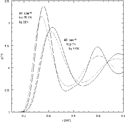
One should use the peak of S_k to decide is a system is solid. For a liquid S_k is smooth and order 1 everywhere. A solid shows a delta functions with peak high a fraction of the number of particles at the reciprocal lattice of the solid. Solid structure shows up in g(r) in a more subtle way: instead of a nice damped oscillations, there are bumps at the nearest neighbor, next-nearest neighbor, etc. (Where they are depends on the type of lattice). See the figures for illustrations of g(r) in liquid helium.

The structure factor also signals separation in a two phase region. An example is the formation of droplets such as occurs when the number of particles corresponds to neither a stable liquid of gas, but a mixture of liquid and gas. In that case the structure function will diverge at low wave vector. The value at zero (S₀) equals N by definition (in the canonical ensemble) but this can be different than limit {k Þ 0} S_k which is proportional to the compressibility of the system.

Order parameters

A key concept from the theory of phase transitions is the idea of an "order parameter" which characterizes a phase. For the moment we will just explain how this works for the two most common phase transitions: liquid-gas and liquid-solid.

The liquid-gas transition: the order parameter is the density. a liquid and gas are identical except a liquid is higher density. At the critical point the difference disappears. There is a first order phase transition between liquid and solid so it is quite possible to do a simulation in the two phase region. What will happen? Liquid droplets will form assuming 1) the surface tension allows it an 2) the simulation is long enough. When this happens Sk will have a characteristic behavior.

The liquid-solid transition : A solid is characterized by a periodic density. For example the Fourier transform of the density will be very large for certain wavevectors (the reciprocal lattice vectors) CLAMPS allows you to input a particular set of vectors to monitor melting and freezing. (keyword READ_K file )

Correlation Functions for Dynamical Response

See the pdf formula page. Readings A & T pgs. 58-64, 185-191

Now consider the calculation of dynamical properties and the response to perturbation. For static properties it would probably be more convenient to do Monte Carlo methods since they are more robust. Dynamics is the reason that we do MD.

The simplest dynamical properties are the linear response to an external perturbation. Most macroscopic measurements are in the linear regime because macroscopic perturbations are very small on the scale of microscopic forces.

Onsager's made a well known conjecture (1935), called the Regression Hypothesis. (also known as the fluctuation-dissipation theorem.) It states that the linear response of the system to a time-varying perturbation is the same as fluctuations that naturally occur in statistical equilibrium. So there are 2 basic ways to calculate response: either wait for the system to fluctuate by itself or apply a perturbation and see what happens. (the first is often referred to as the Kubo method.)

Static perturbation

H = H₀ + c A

where H₀ is the unperturbed Hamiltonian, A is a perturbation and 'c' is the coupling constant. As shown on the formula page one can write the free energy as a power series in 'c'. The linear response is simply the expectation of A in the unperturbed system. The second order term is the fluctuation about the mean. In fact if we neglect all terms above the first order we always get an upper bound to the free energy. Finally to calculate the free energy difference between the system at c=0 and c=1 we just need to integrate the average A over ensembles for various values of c between 0 and 1.

We can also find the response of some property (B) to the perturbation; it equals the correlation between A and B. For example one can find the effect of cutting off the potential. Generally one expects that if the neglected potential is smooth it is pretty much independent of the phase space point R, and hence terms higher order than first can be neglected. A second example is to apply a sinusoidal potential and look at the response of the density. It is simply S _k, the structure factor. That is essentially how neutrons and X-rays measure the structure factor.

Diffusion Constant

The transformation assumes that one is using the unwound coordinates; the positions of the atoms such that:

r(t+h) = r(t) + h v(t) + ...

Don't use periodic boundary conditions to put particles back in the central cell.

One of the key discoveries in the early days of computer simulation was the long-time tails on the v-v function. by Alder and Wainwright. The v-v correlation functions decay algebraically in time. (as t^-d/2) where d is the spatial dimension.) This implies that diffusion may not really exist in 2D. This is not Markovian (random) behavior which would decay exponentially in time. The momentum of a fast moving particle gets stored in the nearby liquid as a vortex and helps to keep it moving in the same direction for a very long time. (citation)

Response to a time varying perturbation

The dynamic structure factor is a key quantity (also known as the density-density response function). If you push the system at time and place (r,t) how does it respond at (r',t')? This is what neutron scattering does. It is not hard to see that sound waves of various kinds will show up as prominent features of S_k (w). This is a good way to see them. The book The Theory of Simple Liquids by Hansen and MacDonald contains a thorough treatment of the theoretical properties of this function.